Are ResNets Antibody Surface Learners?
TLDR: I trained a neural network to predict how much area of each amino acid in an antibody structure can interact with other molecules. The predictor worked really well for amino acids that were buried in the structure but was not as good for highly surface exposed amino acids. This model has future applications in antibody design and engineering.
Introduction
Antibodies are Y-shaped proteins that humans use as a part of the adaptive immune system. Antibodies can identify new foreign invaders in humans and neutralize them with very high specificity. These properties attracted drug hunters and antibodies are currently one of the fastest growing category of medicines with 100 antibody drugs approved by the FDA. Despite all of these successes, the discovery and engineering of therapeutic antibodies rely on many unscalable practices such as immunizing animals with antigens and “guess and check” methods to optimize sequences. Given the prevalence of antibody structural data, computational approaches such as deep learning are promising methods to improve the antibody discovery and engineering process.
Deep learning has recently catalyzed many breakthrough successes in the world of protein structures, replacing physics based models. Until recently, the protein structure prediction world adopted many approaches from the image processing world such as the use of convolutional neural networks and more specifically ResNet architectures (AlphaFold1, Raptor-X, trRosetta). More recently, attention based mechanisms from natural language processing have been used both on unsupervised tasks (TAPE, UniRep etc.) on protein sequences and supervised tasks on protein structures (AlphaFold2).
These advances are extremely exciting but when we want to design new antibody therapeutics we care more about the properties of the molecule than its structure. For example, a good medicine should bind its disease target while also being soluble and not toxic. When considering these secondary characteristics, the physical and chemical properties of amino acids on the surface of the protein are extremely important because they control interactions with other molecules. Currently, these are calculated by bioinformatic pipelines that look for the most similar solved structure and then adapt that structure to make a model called a homology model. This process is time consuming with each sequence taking on the order of minutes to make a model.
Antibodies have a special structure that is slightly different from the use cases of AlphaFold and other structure prediction algorithms. The two upper arms of the Y-shape are called the Fv (or fragment variable) which are responsible for identifying new antigens and binding them. The stalk is called the Fc (fragment crystallizable) and is responsible for attracting other immune cells to destroy the antigen. The Fv specifically is made out of two proteins that associate with eachother called the heavy chain and the light chain (VH and VL respectively). All of these pieces work together in concert to protect us against pathogens!
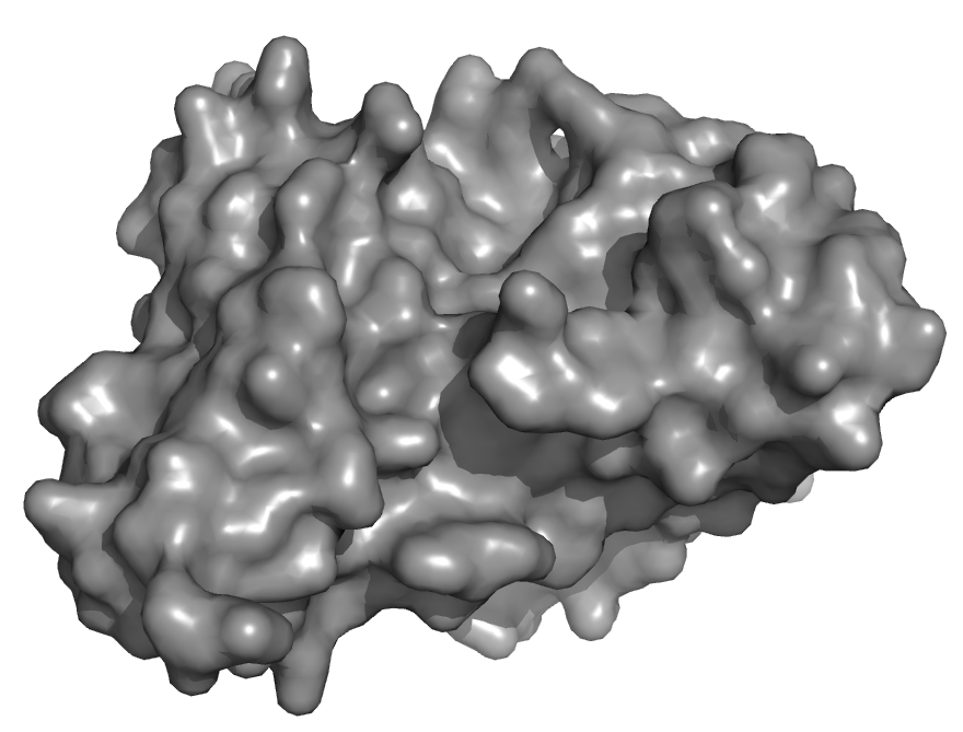
Here, I’m going to describe a small project I did last year that uses a ResNet architecture to predict the solvent exposed surface area (SASA) of each amino acid in a Fv. This approach would be much quicker than building a full homology model and thus allow you to test more potential sequences to find the optimal sequences to test in lab. This has applications in both antibody optimization and could potentially be used in conjunction with other tools to design antibody sequences from scratch on a computer.
Model Architecture
The problem was conceptualized as a classification problem where every amino acid was to be bucketed into one of 25 buckets of normalized SASA values increasing linearly from 0 to 1. The model has 21 1D ResNet blocks with a dropout layer (p=0.2) and a 1d convolutional layer to create the output logits.

Dataset
All structures with a paired VH/VL domain with at most 99% sequence similarity and resolution under 3 Angstroms were selected for dataset. The sequences were truncated to only include the variable region that is known to bind antigens. The sequences in the RosettaAntibody benchmark were removed from the training dataset and used as a test set. Of the remaining structures, 95% of the structures were used as a training set and the remaining set was the validation set. The validation set was never seen during training. The input sequences were one hot encoded with an additional feature indicating where the heavy chain ends and the light chain begins. The SASA values were calculated using the freeSASA python package which used the Shrake-Rupley algorithm which rolls a “ball” over the surface of the structure to find the surface area of each residue that is in contact with the external solvent. The values were normalized to the maximum residue solvent exposure (defined as the exposure of Ala-Xxx-Ala peptide). Any values that were above 1 were set to 1 to prevent the model from learning features about outliers.
Model Training
The model was trained for 30 epochs with a batch size of 4 and the epoch where the training and validation loss were closest was chosen for evaluation. The Adam optimizer was used with an initial learning rate of 0.01 and reduced when the model was plateuing. The outputs were normalized with the Softmax function and the bucket with the highest probability was chosen as the model prediction when evaluating the model against the experimental structures.
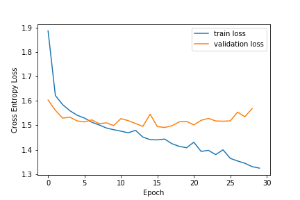
This model was trained with vanilla pytorch on my personal AWS instance on a NVIDIA k80 GPU in about 17 minutes. Inference was also performed on the same machine. I have since migrated to using pytorch lightning for my training to avoid pytorch version and hardware dependency issues.
Overall Model Performance
The model had a 0.45 weighted average precision on the RosettaAntibody benchmark set. The model had significantly higher predictive power on buried positions than exposed positions.
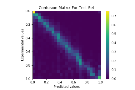
Previous work (Jain et al. (2017) Bioinformatics) on predicting antibody surface areas trained a separate Random Forest Regressor on each residue position in the Fv with handcrafted features. While this approach was accurate, it requires training over 200 models and cannot handle sequences with variable CDR lengths if similar lengths are not found in the training set.
Model Performance on CDR regions
Antibody Fv sequences have a high amount of conservation except for 6 loops, 3 in the heavy chain and 3 in the light chain called complementarity determining regions (CDRs). The CDRs go through rapid evolution which allows them to gain specificity to antigens they have never seen before. Five of the six CDRs adopt some well known folds but the CDRH3 is notoriously difficult to model and specifically important for binding. I calculated the confusion matrices for all the CDRs in the test sets using the Chothia definition.
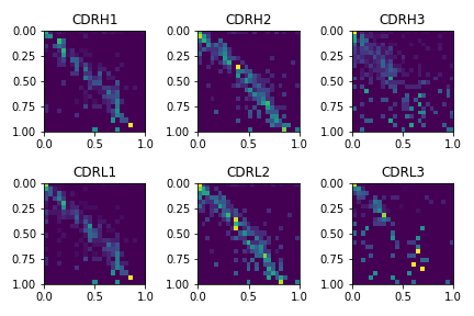
As expected the predictions for the CDRH3 are much worse than the predictions for the other CDRs. The CDRL3 also was harder to model than the other CDRs in the test set. This is a limitation of the method especially in the protein design context because the areas we would design would be the CDRs. Further work with different model architectures might be able to improve the predictions in these CDR regions.
Model Flexibility Predictions
One reason our predictions might be weaker at high solvent exposure is highly solvent exposed residues tend to be more flexible because they have more ability to move around when contacting solvents or other molecules. I hypothesized that the reduction of accuracy for highly solvent exposed residues might actually be taking into account alternative conformations that the protein could take and predicting the protein flexibility as model uncertainty. To test this hypothesis, I looked at the crystallographic B-factors for a structure in our test set which represent how difficult it was to resolve the atoms in the residue. A high B-factor indicates higher flexibility while a lower B-factor indicates less flexibility. This is not a perfect measure of protein flexibility but has been used to identify flexible residues before.
Pseudo-log-likelihood (PLL) is a measure of the joint probability distribution of a collection of random variables. In this case, I used it as a measure of how confident the model is on it’s predictions. Our model is trained with cross entropy loss which tries to maximize the probability of the correct label and the PLL measures the sum of the log probabilities of all the classes.
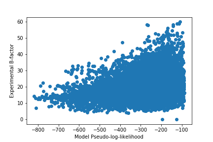
The PLL values seem to broadly indicate that the model had high confidence on many of the rigid positions but seemed to also be confident on some of the more flexible residues. This corresponds with my previous result that the model has better predictive power on buried residues that are probably more rigid than highly exposed residues.
To investigate closer, I chose a case study protein from the test set (PDB ID: 1MFA) where the CDRH3 had low B-factors and a region in the framework had high B-factors to see if the distribution of predicted solvent areas encoded anything about the flexibility of those residues. Since the model performed worse on the CDRH3 region and better on framework regions in general, this will hopefully eliminate the possibility that the distribution of probabilities was due to the model being confused versus it actually learning something about the system.
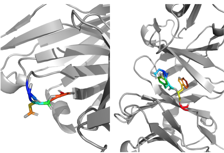
On the left, the framework region with high B-factors. It is a loop region and has multiple prolines and glycines which would indicate that it would be flexible. One the right, the CDRH3 region with low B-factors. This region has bulky residues that might hold it in place and make it more rigid.
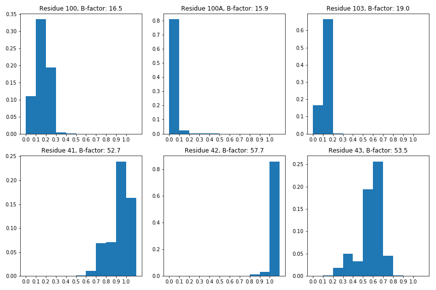
While this is a promising early result, it is hard to conclude that this means that the model has learned about protein flexibility because there are other variables such as the model’s ability to make better predictions for residues with low solvent exposure. While the model’s confidence of predicting solvent exposure at residue 42 is high, residue 42 is a glycine that immediately follows a proline which might mean that both conformations it takes are highly solvent exposed. Further work must be done to conclude that our model is predicting across multiple conformations or just is inaccurate in regions with high solvent exposure.
Future Directions
As mentioned before, there are definitely model architectures that might be able to improve the model accuracy such as including attention mechanisms or appending language model representation features to our hidden states. Additionally, geometric deep learning could be used to learn directly on protein surfaces (point clouds or other graph representations) which might learn interesting features that contribute to protein function. One of the drawbacks of the model architecture chosen is that it is not very interpretable. Interpretable models will be essential to learning new features about proteins or the physical rules that govern folding and activity. For example, a more interpretable model could be more rigorously analyzed to see if the model is learning about flexibility or not.
In principle, this model could also be used for de novo antibody design. If you know what your binding interface looks like, you could in principle fix the solvent exposures of those residues and then search for scaffolds that were likely to stabilize that binding interface. The model could also be used as a feature extractor and be finetuned on experimental data to search the experimental fitness landscape. I did not explore these ideas because I do not have access to a lab to validate any predictions but would be happy to set it up if anyone is interested.
Deep learning is becoming an increasingly powerful tool in the world of structural biology. As we look past the structure prediction problem to the protein design problem, methods that capture features about protein surfaces will be very important to understanding protein and ligand binding pockets, solubility and aggregation which have been difficult to predict with the current methods.
Acknowledgements
Many ideas in this work were influenced by Ruffolo et al. (2020) in Bioinformatics. Thanks to Venkat Munukutla for reading earlier versions of this.